Oops and Optimality
I write a lot of blogposts on why you need more than grid-search to properly judge a machine learning model. In this blogpost I want to demonstrate yet another reason; the optimisers curse.
Dice Analogy
Let's first discuss a game with dice. Let's say that I've got a 100-sided die. I can assume the following;
- If I roll once then the expected value for the number of eyes is 50.5.
- If I roll two times and take the highest of the two then the expected value increases.
- If I roll three times and take the highest of the three then it increases again.
- If I roll four times and take the highest of the four then the it increases yet again.
- etc
Here's the kicker to this situation; it keeps increasing! Every time we roll again we have another opportunity to beat the previous score.
Pretty Distribution
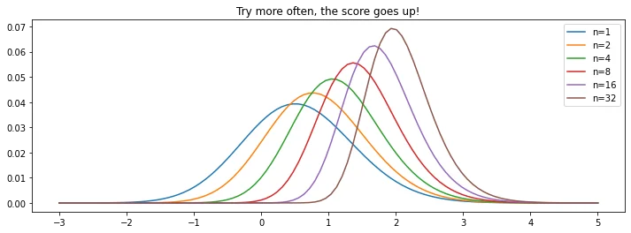
This effect doesn't just hold for dice; it holds for probability distributions in general!
The plot below demonstrates this effect for the normal distribution.
Code.
```python import numpy as np from scipy.stats import norm import matplotlib.pylab as pltplt.figure(figsize=(12, 4)) x = np.linspace(-3, 5, 100) for n in [1, 2, 4, 8, 16, 32]: s = n * norm.pdf(x) * norm.cdf(x)**n plt.plot(x, s/s.sum(), label=f"n={n}")
plt.legend() plt.title("Try more often, the score goes up!");
</details>

<br>

If we really go crazy we can see that the distribution really changes. It's
no longer normally distributed because it is so far skewed to the right.

<figure>
  <img src="pretty-plot2.webp" width="100%" style="margin-left: auto;margin-right: auto;">
  <figcaption>If `n` increases by a lot, it no longer represents the original distribution.</figcaption>
</figure>

<details>
  <summary><b>Code.</b></summary>
import numpy as np from scipy.stats import norm import matplotlib.pylab as plt
plt.figure(figsize=(12, 4)) x = np.linspace(-3, 5, 200) for n in [1, 32, 128, 256, 516]: s = n * norm.pdf(x) * norm.cdf(x)**n plt.plot(x, s/s.sum(), label=f"n={n}")
plt.legend() plt.title("It's getting less and less normal.");
</details>

<br>

## Problem

When we get to "re-roll" before we grab the maximum die then we should expect to see a higher number. This holds for any process with randomness in it. This includes grid-search via cross-validation. Instead of rolling more dice, we can add more parameters to the grid. As we increase the size of the grid, we might start reporting "luck" if we're not careful. W

Cross-validation is not perfectly deterministic. There's noise from the underlying algorithm, numeric in-accuracies as well as the cross-validation itself.
And I'm not even talking about using the [random seed as a hyperparameter](https://twitter.com/beenwrekt/status/913418862191710208?lang=en).

So let's see if we can quantify this effect using an actual example.

## Creditcard

Let's grab the [creditcard](https://www.kaggle.com/jacklizhi/creditcard) dataset and try to predict some fraud. This dataset is available directly via [scikit-lego](https://scikit-lego.readthedocs.io/en/latest/datasets.html#Fetch-creditcard).
from sklego.datasets import fetch_creditcard
from sklearn.model_selection import GridSearchCV from sklearn.linear_model import LogisticRegression from sklearn.metrics import make_scorer, accuracy_score
X, y = fetch_creditcard(return_X_y=True)
def run_grid(settings=10, cv=5): params = { 'C': np.linspace(.1, 10.0, settings) }
grid = GridSearchCV(
    estimator=LogisticRegression(class_weight="balanced"),
    cv=cv,
    n_jobs=-1,
    param_grid=LogisticRegression,
    scoring={"acc": make_scorer(accuracy_score)},
    refit="acc"
)

return pd.DataFrame(grid.fit(X, y).cv_results_).sort_values("rank_test_acc");
This code-block gives us a function `run_grid` that runs a grid-search. We are optimising a parameter `C` which represents regularisation strength and we can choose to consider many settings for that parameter or few. We also have a `cv` argument that allows us to specify how many cross-validations to perform.

I've been running this function with a whole bunch of settings and it eventually was able to give me this data.

|settings/cv |        2 |        5 |
|-----------:|---------:|---------:|
|          5 | 0.944102 | 0.973533 |
|         10 | 0.94695  | 0.973705 |
|         20 | 0.945184 | 0.973810 |
|        100 | 0.956050 | 0.974150 |

There's a few things to point out here.

First, calculating this takes a fair amount of time, even on this relatively small dataset. If we try out 100 parameters and cross validate five times then waiting becomes part of our job.

Second, if you want higher grid-search results it might help to increase the number of cross-validations that you make. I might argue that methodologically this not a "super bad" observation. It means that you might need to spend a lot of compute resources but it makes sense. If you only have 2 sets for cross validation then the model only learns from 1/2 of the dataset. If you have 5 sets then the model can learn from 4/5 of the dataset and should therefore generalise better.

Thirs, if you want higher grid-search results; it seems good to increase the size of the grid. But let's think twice about what this means. Are we seeing this because of a better hyperparameter? Or is this the "more-dice" effect?

<figure>
  <img src="assumptions.webp" width="100%" style="margin-left: auto;margin-right: auto;">
  <figcaption>In other words; can we really trust these sorts of statements?</figcaption>
</figure>

## Checking

Let's zoom in on that one grid-search that is *big* and has 100 settings. We'll first look at the top grid-search results.

|   rank_test_acc |   param_C |   mean_test_acc |
|----------------:|----------:|----------------:|
|               1 |       0.8 |        0.974151 |
|               2 |       7.8 |        0.973705 |
|               3 |       5.1 |        0.973589 |
|               4 |       9.8 |        0.973512 |
|               5 |       0.1 |        0.973473 |


Is it just me, or does this look fishy? The best scoring `param_C` values here don't seem to be related to `mean_test_acc`. In fact, they're spread all across the spectrum. You'd expect the best scoring candidates to be similar and different to the rest. This begs the question; is there a relationship between the `param_C` values that we're considering and the test score? Let's plot it.

<figure>
  <img src="randomness.webp" width="100%" style="margin-left: auto;margin-right: auto;">
  <figcaption>This is noise.</figcaption>
</figure>

I don't know about you, but this looks like random data to me. The best score that we're selecting, might just get picked due to luck, not because it is contributing to a better model.

## What is Happening?

The example here is a bit silly. This dataset is very imbalanced which is making it hard for the `LogisticRegression` to properly converge. The parameter `C` therefore isn't contributing much. That means that by optimising for it, you're more likely capturing noise than measuring the contribution that it makes to predictive power.

But the point isn't the dataset. It's the fact that `GridSearchCV` has no way to deal with this extra noise. It will just pick the best model according to the score that we provide it. The only way to understand that we're optimising for noise here is to understand the data and the model in our system. You shouldn't call `fit(X, y).predict(X)` and call it a day. You need more.

Think about this if you're running a big grid-search on a daily basis. If you blindly give your `EnterpriseAutoML[tm]`-engine a gigantic set of parameters to go optimise for, and you find a new model reported to be 0.15% better are you sure it's really better? You're probably not making the model better, instead you're optimising for the noise of your cross-validation. This is dangerous territory because you might report overly optimistic numbers which will dissapoint everyone when the model is deployed.

Not to mention all the compute power you've wasted.

## Conclusion

Grid-search is not a inheritly bad idea. In fact, there's many merits to it! The main point here is to demonstrate that it is not enough. You can game it by artificially inflating the parameter grid.

In this blogpost we've shown a phenomenon called "the optimisers curse." The odds of getting too optimistic during optimisation increases the more cases you consider. The problem isn't a high statistic in a table, the problem is that that number doesn't represent what will happen in reality.

!!! quote "Appendix"

    If you want to learn more about the optimisers curse you can check [the original paper](http://tuck-fac-cen.dartmouth.edu/images/uploads/faculty/james-smith/The_Optimizers_Curse.pdf).

    If you're interested in fiddling around with the notebook, you can find the scratchpad [here](optimizers_curse.ipynb).