Vary Very Optimally
This document was inspired by this blogpost by Ferenc Huszár which was in turn inspired by this paper by Wiersta et al and this paper by Barber et al. I was a fascinated by all of this and I just had to reproduce it myself. I'm sharing some personal findings based on that work here but any proper attribution should also link to the previously mentioned documents as I am largely just repeating their work.
Problem of Hard Functions
Sometimes we are interested in optimising functions that are hard to optimise. This happens often in machine learning but also in decision science. Here are two examples of functions ($\text{sinc}(x)$ and $\lfloor 10\text{sinc}(x) + 4\sin(x)\rfloor$) that could be seen as hard.
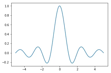

Both functions have mulitiple peaks which makes them hard to approach via gradient descent. To make things worse, the right chart is not differentiable and has a very thin peak at the top which is hard to find.
Instead of searching in a one dimensional space though, how about apply a smoothing factor and turn the gradient descent from a one dimensional problem into a two dimensional problem?
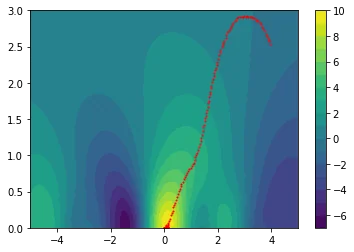
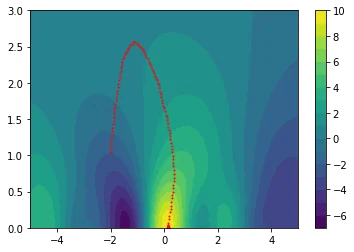
The plots below translate our original one-dimensional hard functions into easier two-dimensional spaces.
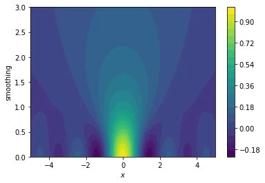
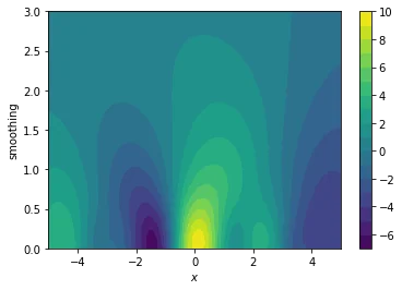
We'll explain how the smoothing works in just a bit but try to pay close attention to what the consequences are of such a smoothed space:
- we are now optimising a landscape $g(x,s)$ where $s$ is the amount of smoothing we apply
- when $s=0$ then we define $g(x, 0) = f(x)$
- when $s>>0$ then $g(x, s)$ starts to resemble an average of sorts
- if we start a gradient descent algorithm in a region where the smoothing parameter is high it is likely that we move towards the actual optimum of a region
- if we start a gradient descent algorithm in a region where $s \approx 0$ then we are also able to escape the local optima because the gradient search might be interested in searching in a space where $s$ is larger
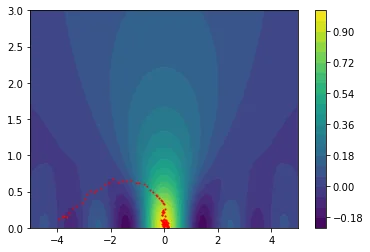
The plots below show how the gradient descent in this space causes us to avoid local optima.

I hope that by now, we're all very exited about this special smoother.
How to Smooth
There are many ways to look at our special smoother. Some people might call it a convolution while others might call it a variational bound. Before delving into the maths of it, I'll first discuss the idea with images and intuition.
Intuition
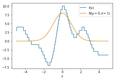
Step 1
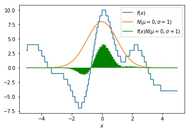
The idea is that we take our original function $f(x)$ (blue) and we smoothe it around some value of $x$ with a gaussian that is distributed $N(\mu=x, \sigma)$ (orange). In the example here we take $\mu=x=0$ and $\sigma=1$. Note that the orange line is not drawn to scale, but we need it to illustrate a point.
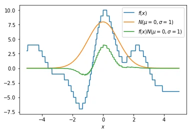
Step 2
The idea now is that we smooth our function $f(x)$ by multiplying it by the distribution of $N(\mu=x=0, \sigma=1)$. Points that are closer to $x$ will have more influence on the smoothed value, especially when $\sigma$ is small. We now plot the $f(x)N(\mu, \sigma)$ with a green line. Notice that it indeed seems to smoothe our original $f(x)$ function.
Step 3
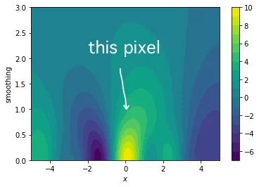
This green line is cool and all, but we would like this green line to be summarised into a single number. We are looking for a two dimensional function with a smoothing factor $s$ and an $x$ value such that we can perform gradient descent on it. How about we integrate the green area that exists between the green line and the x-axis? That area can be interpreted as a gaussian average of $f(x)$ given $\sigma$.
Step 4
The integral we just calculated is the value we find in our gradient search space at $x=0$ and $\sigma=1$. I've drawn the location of this pixel in the image to emphesize. Typically we don't need to generate the entire search space though, we merely need to be able to sample from it for our gradient.
Effect
It helps to look at things from different perspectives so let's double check what the effect of our smoothing parameter $\sigma$ is on the function that we are performing a grid search on.
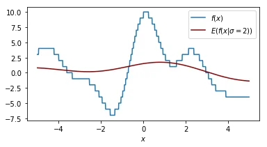
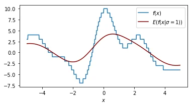
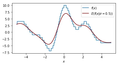
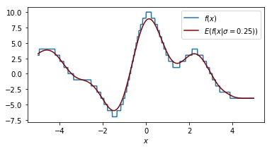
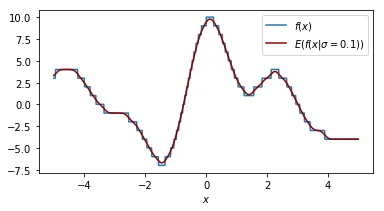
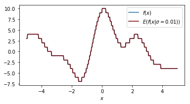
Each plot shown shows the original function in blue and the smoothed function in dark red. The plot shows similar information as the 2d plot we saw in step 4 but this plot assumes that the smoothing factor is constant. You can see that when the smoothing factor increases we smoothe all the values closer to zero but we still have a glimpse of the actual value.
Another way of thinking about this smoothing function is that it is an approximation of our original function.
Enter Maths
The maths surrounding this topic feel like poetry to me, but feel free to skip it if this doesn't apply to you.
Our gaussian average can be seen as an estimator for the original function $f(x)$. It is the expected value of $f(x)$ given a value of $\mu$ and $\sigma$.
$$ \min f(x) \leq \min \mathbb{E}_{x \sim p(x|\mu, \sigma)}[f(x)] = \min g(\mu, \sigma, f)$$
The idea is that we optimise $g(\mu, \sigma, f)$ which will serve as an upper bound for $f(x)$. This means that if we are able to perform a proper gradient search of $g$ then we should be able to find interesting candidates for optimal values of $f(x)$.
This means we need to do some maths surrounding the gradient. Let's combine our $\mu$ and $\sigma$ into a single parameter $\theta$. Then;
$$
\begin{split}
\frac{d}{d\theta} \mathbb{E}_{x \sim p(x|\theta)} f(x) &= \frac{d}{d\theta}\int p(x|\theta)f(x)dx \\
&= \int \frac{d}{d\theta} p(x|\theta)f(x)dx
\end{split}
$$
So far so good. Let's now apply a trick. We will rewrite the contents of the last integral in a bit. To understand why we are able to do that, please remember the chain rule of derivatives;
$$ \frac{d}{dx} f(g(x)) = g'(x) f'(g(x)) $$
We will now apply the chain rule on the following statement.
$$ \frac{d}{d\theta} \log p(x|\theta) = \frac{\frac{d}{d\theta}p(x|\theta)}{p(x|\theta)} $$
You may begin to wonder why this is such a useful step. Hopefully it comes clear when we multiply both sides by $p(x|\theta)$.
$$
\begin{split}
\frac{d}{d\theta} \log p(x|\theta) & = \frac{\frac{d}{d\theta}p(x|\theta)}{p(x|\theta)} \\
p(x|\theta) \frac{d}{d\theta} \log p(x|\theta) & = p(x|\theta) \frac{\frac{d}{d\theta}p(x|\theta)}{p(x|\theta)} \\
p(x|\theta) \frac{d}{d\theta} \log p(x|\theta) & = \frac{d}{d\theta} p(x|\theta)
\end{split}
$$
Let us now use this to continue our train of thought.
$$
\begin{split}
\frac{d}{d\theta} \mathbb{E}_{x \sim p(x|\theta)} f(x) &= \frac{d}{d\theta}\int p(x|\theta)f(x)dx \\
&= \int \frac{d}{d\theta} p(x|\theta)f(x)dx \\
&= \int p(x|\theta)\frac{d}{d\theta} \log p(x|\theta)f(x)dx
\end{split}
$$
That seems useful, let's rearrange and conclude!
$$
\begin{split}
\frac{d}{d\theta} \mathbb{E}_{x \sim p(x|\theta)} f(x) &= \frac{d}{d\theta}\int p(x|\theta)f(x)dx \\
&= \int \frac{d}{d\theta} p(x|\theta)f(x)dx \\
&= \int p(x|\theta)\frac{d}{d\theta} \log p(x|\theta)f(x)dx \\
&= \int p(x|\theta) f(x) \frac{d}{d\theta} \log p(x|\theta)dx \\
&= \mathbb{E}_p \left< f(x) \frac{d}{d\theta} \log p(x|\theta) \right>
\end{split}
$$
The implications of this are pretty interesting because we are very open to whatever function $f(x)$ that we come up with. Also, if we want to estimate the gradient we do not need to calculate the full integral of the expected value; we could also sample it instead. Imagine that we sample lot's and lot's of $x_s \sim p(x^s|\theta)$ then we can write the gradient update rule as (assuming maximisation):
$$\theta^{\text{new}} = \theta + \frac{\alpha}{S} \sum_S f(x^s) \frac{d}{d\theta} \log p(x^s|\theta)$$
Furthermore; we are free to pick whatever smoothing distribution we want but if we pick the gaussian distribution such that $\theta = {\mu, \Sigma}$ we gain some nice closed from solutions.
$$
\begin{bmatrix} \mu \\ \Sigma \ \end{bmatrix}^{\text{new}}
= \begin{bmatrix} \mu \\ \Sigma \\\end{bmatrix}
+ \frac{\alpha}{S} \sum_S f(x^s)
\begin{bmatrix}
\Sigma^{-1}(x^s-\mu) \\
-\frac{1}{2}(\Sigma^{-1} - \Sigma^{-1}(x^s-\mu)(x^s-\mu)^T\Sigma^{-1}) \\
\end{bmatrix}
$$
If you are interested in proofs like these, google "Matrix Cookbook". I didn't come up with these and neither should you.
Python Code
To proove that this works I've written some python code that rougly applies the maths we've just discussed.
def formula_update_orig(f, mu, sigma, alpha=0.05, n=50, max_sigma=10):
    mu_arr = np.array(mu).reshape(2)
    dmu, dsigma = np.zeros(shape=mu.shape).T, np.zeros(shape=sigma.shape)

    for i in range(n):
        xs = np.random.multivariate_normal(mu_arr, sigma)
        inv_sigma = np.linalg.inv(sigma)
        dmu += np.matrix(alpha/n * f(xs) * inv_sigma * (xs-mu).T)
        sigma_part = -alpha/n * f(xs)*(inv_sigma - inv_sigma*(xs-mu).T*(xs-mu)*inv_sigma)/2
        dsigma += sigma_part

    new_mu = (mu.T + dmu).reshape((1,2))
    new_sigma = sigma + dsigma

    # now comes the dirty numerics to prevent numerical explosions
    new_sigma[new_sigma > max_sigma] = max_sigma
    new_sigma[new_sigma > sigma*2] = 0.1
    new_sigma[new_sigma < 0.05] = 0.05
    return new_mu, new_sigma
The code has some dirty parts because of numerical stability but it serves it's purpose in demonstrating that we are able to use this tactic on higher dimensional functions too.
Higher Dimensions
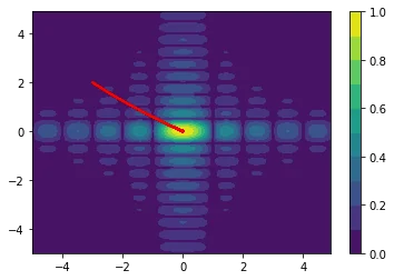
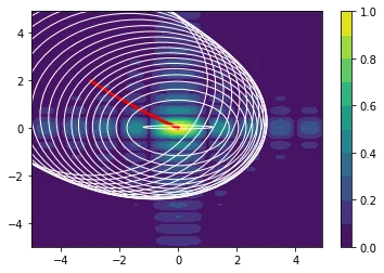
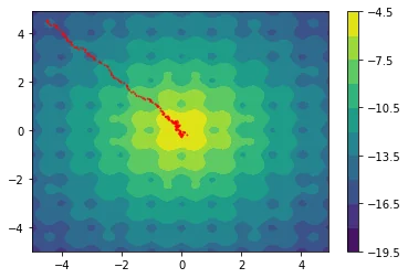
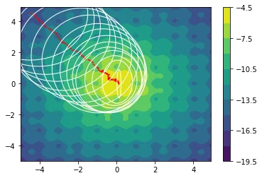
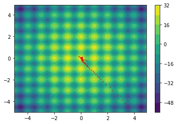
The following examples are all two dimensional functions. We plot the actual two dimensional space without any smoothing parameters to show that our method also works in higher dimensions. For every function we see three charts. The first chart is the actualy search space, the second chart contains the search space with the gradient path and the first chart also includes the search space that is defined by $\Sigma$.
$$f(x,y) = \sqrt{|\text{sinc}(2x)| * |\text{sinc}(y)|}$$
$$ f(x,y) = -20\text{exp}\left(-0.2*\sqrt{(0.5*(x^2 + y^2))}\right) + \text{exp}\left(0.5\cos(2 \pi x) + \cos(2 \pi y)\right)$$
$$ f(x,y) = 10 - x^2 - x^y - 10 * \cos(2 \pi x) - 10 * \cos(2 \pi y)$$
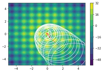
Note that the algorithm automatically sweeps the area and converges when it seems that it cannot find better regions.
Conclusions {.appendix}
Although this trick has very pleasing maths to it, there's a few things that are still worth to note;
- Although this trick seems like a viable tactic against local optima we haven't been given a guarantee of optimality with this approach. If we start our search at the wrong end of the search spectrum with a small $\sigma$ we are prone to still get stuck in a local optima.
- When we increase the dimensionality of our search problem we will also need to increase the amount of samples that we need per gradient step otherwise we risk a bit of bias in our gradient estimation.
- We are able to parallize parts of the sampling that we do. If each process has a different sampling seed then we can run part of the sampling in parallel.
- Improper parameter tuning is still a potential road to ruin. If the stepsize is too large the system can be very unstable.
- The approach feels similar to the evolutionary strategies heuristic and simulated annealing except that we've thrown a lot of extra maths in the mix such that we're able to search in our variance/temperature space as well. One can imagine that ES and SA to also have reasonable results on the problems we've tried.
- This method of optimisation seems to be worthwhile if you've got a very peaky search space but one that is cheap to evaluate. If it takes a long time to evaluate a function it may be better to try out bayesian optimisation tactics or hyperopt instead.
If you want to play with the messy notebook that I used for this blogpost, feel free to play with it.